gephi – OUseful.Info, the blog…

Getting Started With The Gephi Network Visualisation App – My Facebook Network, Part I

A couple of weeks ago, I came across Gephi, a desktop application for visualising networks.

And quite by chance, a day or two after I was asked about any tools I knew of that could visualise and help analyse social network activity around an OU course… which I take as a reasonable justification for exploring exactly what Gephi can do :-)

So, after a few false starts, here’s what I’ve learned so far…

First up, we need to get some graph data – netvizz – facebook to gephi suggests that the netvizz facebook app can be used to grab a copy of your Facebook network in a format that Gephi understands, so I installed the app, downloaded my network file, and then uninstalled the app… (can’t be too careful ;-)

Once Gephi is launched (and updated, if it’s a new download – you’ll see an updates prompt in the status bar along the bottom of the Gephi window, right hand side) Open… the network file you downloaded.

NB I think the graph should probably be loaded as an undirected graph… That is, if A connects to B, B connects to A. But I’m committed to the directed version in this case, so we’ll stick with it… (The directed version would make sense for a Twitter network (which has an asymmetric friending model), where A may follow B, but B might choose not to follow A. In Facebook, friending is symmetric – A can only friend B if B friends A.

(Btw, I’ve come across a few gotchas using Gephi so far, including losing the window layout shown above. Playing with the Reset Windows from the Windows menu sometimes helps… There may be an easier way, but I haven’t found it yet…)

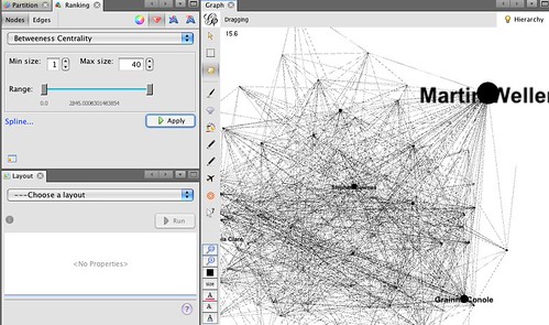
The graph window gives a preview of the network – in this case, the nodes are people and the edges show that one person is following another. (Remember, I should have loaded this as an undirected graph. The directed edges are just an artefact of the way the edge list that states who is connected to whom was generated by netvizz.)

Using the scroll wheel on a mouse (or two finger push on my Mac mousepad), you can zoom in and out of the network in the graph view. You can also move nodes around, view the labels, switch the edges on and off off, and recenter the view.

Not shown – but possible – is deleting nodes from the graph, as well as editing their properties.

You can also generate views of the graph that show information about the network. In the Ranking panel, if you select the Nodes tab, set the option to Degree (the number of edges/connections attached to a node) and then choose the node size button (the jewel), you can set the size of the node to be proportional to the number of connections. Tune the min and max sizes as required, then hit apply:

You can also colour the nodes according to properties:

So for example, we might get something like this:

Label size and colour can also be proportional to node attributes:

To view the labels, make sure you click on the Text labels option at the bottom of the graph panel. You may also need to tweak the label size slider that’s also on the bottom of the panel.

If you want to generate a pretty version of the graph, you need to do a couple of things. Firstly, in the layout panel, select a layout algorithm. Force Atlas is the one that the original tutorial recommends. The repulsion strength determines how dispersed the final graph will be (i.e. it sets the “repulsive force” between nodes); I set a value of 2000, but feel free to play:

When you hit Run, the button label will change to Stop and the graph should start to move and reorganise itself. Hit Stop when the graph looks a little better laid out. Remember, you can also move nodes around in the graph as show in the video above.

Having run the Layout routine, we can now generate a pretty view of the graph. In the Preview Settings panel on the left-hand side of the Gephi environment, select “Show Labels” and then hit “Refresh”:

In the Preview panel, (next tab along from Preview Settings), you should see a the prettified, 3D layout view:

Note that in this case I haven’t made much attempt at generating a nice layout, for example by moving nodes around in the graph window to better position them, but you can do… (just remember to Refresh the Preview view in the Preview Settings… (There must be a shortcut way of doing that, but I haven’t found it…!:-(

If you want to look at who any particular individual is connected to, you can go to the
Data Table panel (again in the set of panels on the right hand side, just along from the Preview tab panel) and search for people by name. Here, I’m searching the edges to see who of my Facebook friends a certain Martin W is also connected to on Facebook;

It’s easy enough to highlight/select and copy these cells and then post them into a spreadsheet if required.

So that’s step 1 of getting started with Gephi… a way of using it to explore a graph in very general terms; but that’s not where the real fun lies. That starts when you start processing the graph by running statistics and filters over it. But for that, you’ll have to wait for the next post in this series… which is here: Getting Started With Gephi Network Visualisation App – My Facebook Network, Part II: Basic Filters

Getting Started With Gephi Network Visualisation App – My Facebook Network, Part II: Basic Filters

In Getting Started With Gephi Network Visualisation App – My Facebook Network, Part I I described how to get up and running with the Gephi network visualisation tool using social graph data pulled out of my Facebook account. In this post, I’ll explore some of the tools that Gephi provides for exploring a network in a more structured way.

If you aren’t familiar with Gephi, and if you haven’t read Part I of this series, I suggest you do so now…

…done that…?

Okay, so where do we begin? As before, I’m going to start with a fresh worksheet, and load my Facebook network data, downloaded via the netvizz app, into Gephi, but as an undirected graph this time! So far, so exactly the same as last time. Just to give me some pointers over the graph, I’m going to set the node size to be proportional to the degree of each node (that is, the number of people each person is connected to).

I can activate text labels for the nodes that are proportional to the node sizes from the toolbar along the bottom of the Graph panel:

…remembering to turn on the text labels, of course!

So – how can we explore the data visually using Gephi? One way is to use filters. The notion of filtering is incredibly powerful one, and one that I think is both often assumed and underestimated, so let’s just have a quick recap on what filtering is all about.

This maybe?

[“green beans” by House Of Sims]

Filters – such as sieves, or colanders, but also like EQ settings and graphic, bass or treble equalisers on music players, colour filters on cameras and so on – are things that can be used to separate one thing from another based on their different properties. So for example, a colander can be used to separate green beans from the water it was boiled in, and a bass filter can be used to filter out the low frequency pounding of the bass on an audio music track. In Gephi, we can use filters to separate out parts of a network that have particular properties from other parts of the network.

The graph of Facebook friends that we’re looking at shows people I know as nodes; a line connecting two nodes (generally known as an edge) shows that that the two people represented by the corresponding nodes are also friends with each other. The size of the node depicts its degree, that is, the number of edges that are connected to it. We might interpret this as the popularity (or at least, the connectedness) of a particular person in my Facebook network, as determined by the number of my friends that they are also a friend of.

(In an undirected network like Facebook, where if A is a friend of B, B is also a friend of A, the edges are simple lines. In a directed network, such as the social graph provided by Twitter, the edges have a direction, and are typically represented by arrows. The arrow shows the direction of the relationship defined by the edge, so in Twitter an arrow going from A to B might represent that A is a follower of B; but if there is no second arrow going from B to A, then B is not following A.)

We’ve already used degree property of the nodes to scale the size of the nodes as depicted in the network graph window. But we can also use this property to filter the graph, and see just who the most (or least) connected members of my Facebook friends are. That is, we can see which people are friends of lots of the people am I friends of.

So for example – of my Facebook friends, which of them are friends of at least 35 people I am friends with? In the Filter panel, click on the Degree Range element in the Topology folder in the Filter panel Library and drag and drop it on to the Drag Filter Here

Adjust the Degree Range settings slider and hit the Filter button. The changes to allow us to see different views over the network corresponding to number of connections. So for example, in the view shown above, we can see members of my Facebook network who are friends with at least 30 other friends in my network. In my case, the best connected are work colleagues.

Going the other way, we can see who is not well connected:

One of the nice things we can do with Gephi is use the filters to create new graphs to work with, using the notion of workspaces.

If I export the graph of people in my network with more than 35 connections, it is place into a nw workspace, where I can work on it separately from the complete graph.

Navigating between workspaces is achieved via a controller in the status bar at the bottom right of the Gephi environment:

The new workspace contains just the nodes that had 35 or more connections in the original graph. (I’m not sure if we can rename, or add description information, to the workspace? If you know how to do this, please add a comment to the post saying how:-)

If we go back to the original graph, we can now delete the filter (right click, delete) and see the whole network again.

One very powerful filter rule that it’s worth getting to grips with is the Union filter. This allows you to view nodes (and the connections between them) of different filtered views of the graph that might otherwise be disjoint. So for example, if I want to look at members of my network with ten or less connections, but also see how they connect to each other to Martin Weller, who has over 60 connections, the Union filter is the way to do it:

That is, the Union filter will display all nodes, and the connections between them, that either have 10 or less connections, or 60 or more connections.

As before, I can save just the members of this subnetwork to a new workspace, and save the whole project from the File menu in the normal way.

Okay, that’s enough for now… have a play with some of the other filter options, and paste a comment back here about any that look like they might be interesting. For example, can you find a way of displaying just the people who are connected to Martin Weller?

Getting Started With Gephi Network Visualisation App – My Facebook Network, Part III: Ego Filters and Simple Network Stats

In a couple of previous posts on exploring my Facebook network with Gephi, I’ve shown how to plot visualise the network, and how to start constructing various filtered views over it (Getting Started With The Gephi Network Visualisation App – My Facebook Network, Part I and Getting Started With Gephi Network Visualisation App – My Facebook Network, Part II: Basic Filters). In this post, I’ll explore a new feature, ego filters, as well as looking at some simple social network analysis tools that can help us better understand the structure of a social network.

To start with, I’m going to load my Facebook network data (grabbed via the Netvizz app, as before) into Gephi as an undirected graph. As mentioned above, the ego network filter is a new addition to Gephi, which will show that part of a graph that is connected to a particular person. So for example, I can apply the ego filter (from the Topology folder in the list of filters) to “George Siemens” to see which of my Facebook friends George knows.

If I save this as a workspace, I can then tunnel into it a little more, for example by applying a new ego filter to the subgraph of my friends who George Siemens knows. In this case, lets add Grainne to the mix – and see who of my friends know both George Siemens and Grainne:

Note that I could have achieved a similar effect with the full graph by using the intersection filter (as introduced in the previous post in this series):

The depth of the ego filter also allows you to see who of of my friends the named individual knows either directly, or through one of my other friends. Using an ego filtered network to depth two (frined of a friend) around George Siemens, I can run some network statistics over just that group of people. So for example, if I run the Degree statistics over the network, and then set the node size according to node degree within that network this is what I get:

(I also turned node labels on and set their size proportional to node size.)

Running Network Diameter stats generates the following sorts of report:

That is:

– betweenness centrality;
– closeness centrality;
– eccentricity.

These all sound pretty technical, so what do they refer to?

Betweenness centrality is a measure based on the number of shortest paths between any two nodes that pass through a particular node. Nodes around the edge of the network would typically have a low betweenness centrality. A high betweenness centrality might suggest that the individual is connecting various different parts of the network together.

Closeness centrality is a measure that indicates how close a node is to all the other nodes in a network, whether or not the node lays on a shortest path between other nodes. A high closeness centrality means that there is a large average distance to other nodes in the network. (So a small closeness centrality means there is a short average distance to all other nodes in the network. Geddit? (I think sometimes the reciprocal of this measure is given as closeness centrality:-).

The eccentricity measure captures the distance between a node and the node that is furthest from it; so a high eccentricity means that the furthest away node in the network is a long way away, and a low eccentricity means that the furthest away node is actually quite close.

So let’s have a look at the structure of my Facebook network, as filtered according to George’s ego filter, depth 2:

Plotting size proportional to betweenness centrality, we see Martin Weller, Grainne and Stephen Downes are influential in keeping different parts of my network connected:

As far as outliers go, we can look at the closeness centrality and eccentricity (to protect the innocent, I shall suppress the names!)

Here, the colour field defines the closeness centrality and the size of the node the eccentricity. It’s quite easy to identify the people in this network who are not well connected and who are unlikely to be able to reach each other easily through those of my friends they know.

From nods with similar sizes and different colours, we also see how it’s quite possible for two nodes to have a similar eccentricity (similar distances to the furthest away nodes) and very different closeness centrality (that is, the node may have a small or large average distance to every other node in the graph). For example, if a node is connected to a very well connected node, it will lower the closeness centrality.

So for example, if we look at the ego network with the above netwrok based around the very well connected Martin Weller, what do we see?

The colder, blue shaded circles (high closeness centrality) have disappeared. Being a Martin Weller friend (in my Facebook network at least) has the effect of lowering your closeness centrality, i.e. bringing you closer to all the other people in the network.

Okay, that’s definitely more than enough for now. Why not have a play looking at your Facebook network, and seeing if you can identify who the best connected folk are?

PS when plotting charts, I think Gephi uses data from the last statistics run it did, even if that was in another workspace, so it’s always worth running the statistics over the current graph if you intend to chart something based on those stats…

Getting Started With The Gephi Network Visualisation App – My Facebook Network, Part V

A comment from one of the Gephi developers to Getting Started With The Gephi Network Visualisation App – My Facebook Network, Part IV, in which I described how to use the Modularity statistic to partition a network in terms of several different similar subnetwork groupings, suggested that a far better way of visualising the groups was to use the Partion parameter… and how right they were…

Running the Modularity statistic over my Facebook netwrok, as captured using Netvizz, and then refreshing the view in the Partition panel allows us to colour the netwrok using different partitions – such as the Modularity classes that the Modularity statistic generates and assigns nodes to:

Here’s what happens when we applying the colouring:

Selecting the Group view collects all the nodes in a partition together as a group:

These grouped nodes can be individually ungrouped by right-clicking on a group node and ungrouping it, or they can be expanded which maintains the group identity whilst still letting us look at the local structure:

Here’s what the expanded view of one of the classes looks like, with text labels turned on:

We see that the members of the group are visible, allowing us to explore the make-up of the subnetwork. As you might expect, we can then colour or resize nodes within the expanded group in the normal way:

To create a workspace containing just the members of a particular partition, ungroup all the nodes via the Partition module and filter on the required partition using a Modularity Class filter:

The Partition module is incredibly powerful, as you can hopefully see; but it isn’t limited to dealing with just partitions created using Gephi statistics – it can also deal with partitions defined over the graph as loaded into Gephi (see the GUESS format for more details on how to structure the input file).

So for example, the most recent version of Netvizz will return additional data alongside just the identities of your friends, such as their gender (if revealed to you by their profile privacy settings) and the number of their wall posts. Loading this richer network specification into Gephi, and refreshing the Partion module settings reveals the following: